How to Make Models Reason with GRPO

26 March 2025 - 13 mins read time
Tags: research RL

How to Make Model “Reason” with Group Relative Policy Optimization (GRPO)

You’ll notice that ChatGPT has a small “Reasoning” button under the prompt and see that it suddenvly significantly “evolves” into a more powerful version that can math and coding problem well. Given the recent rise of reasoning powered LLMs, such as OpenAI’s o1 and o3 and DeepSeek’s R1, and some might get curious on how these models are created and trained.

These questions can be:

What is the methodology to train such reasoning models?
What difference does it have compared to traditional LLM training process?

In this blog, we will explore the foundational blocks of training/tuning an LLM model to reason and try to answer questions we discussed earlier. The topics would roughly include:

Introduction to Reinforcement Learning
Policy in Reinforcement Learning
PPO (Proximal Policy Optimization)
GRPO (Group Relative Policy Optimization)

Reinforcement Learning in Post-Training LLMs

In the context of training an LLM, we normally think of pretraining -> finetuning -> RLHF (reinforcement learning with human feedback). The latter parts of the LLM training process are called post-training (i.e. the process after pretraining).

Basically, reinforcement learning is a process of teaching an agent, which can be a language model or any other modality model, on how to behave (take which action) in a given environment setting to maximize certain reward.

Think of how we learn from our past experiences. This can be lessons learned from our mistakes and successes. Through each outcome of our actions, we get certain reward- or punishment (we’ll refer to this as negative or positive feedback). So reinforcement learning is a very natural way of teaching an agent, though the environment is “a bit” more restrained like a sandbox, compared to our real open world.

What’s more interesting about reinceforcement learning, especially when comparing it to machine learning (supervised, using labeled dataset), is that we are not necessarily supervising the model- or an “agent” as we normally refer to in the reinforcement context. We are leaving the agent to learn by itself on how to maximize the reward for every action it takes. The goal is not to micromanage- by telling our baby agent what you did was good or bad- instead, let it observe the outcome itself and learn the best action (let it decide) for each environment state given.

alt text

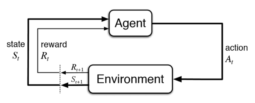
Refer to this flow diagram. The process of reinforcement learning goes like this. Focus!

Our agent that we want to train receives an environment “state,” denoted as \(S_t\) at time \(t\).
Based on the state \(S_t\), the agent will take a certain action, denoted as \(A_t\).
Now, that action will have an impact on the state, which will create a new state of the environment, \(S_{t+1}\).
Based on the action and the new state, a new reward, \(R_{t+1}\), is calculated- which will influence how the agent will act in subsequent steps.
Repeat steps 1-4, but for \(t>0\), the agent receives the environment state and reward instead of just the environmnt on \(t=0\).

alt text

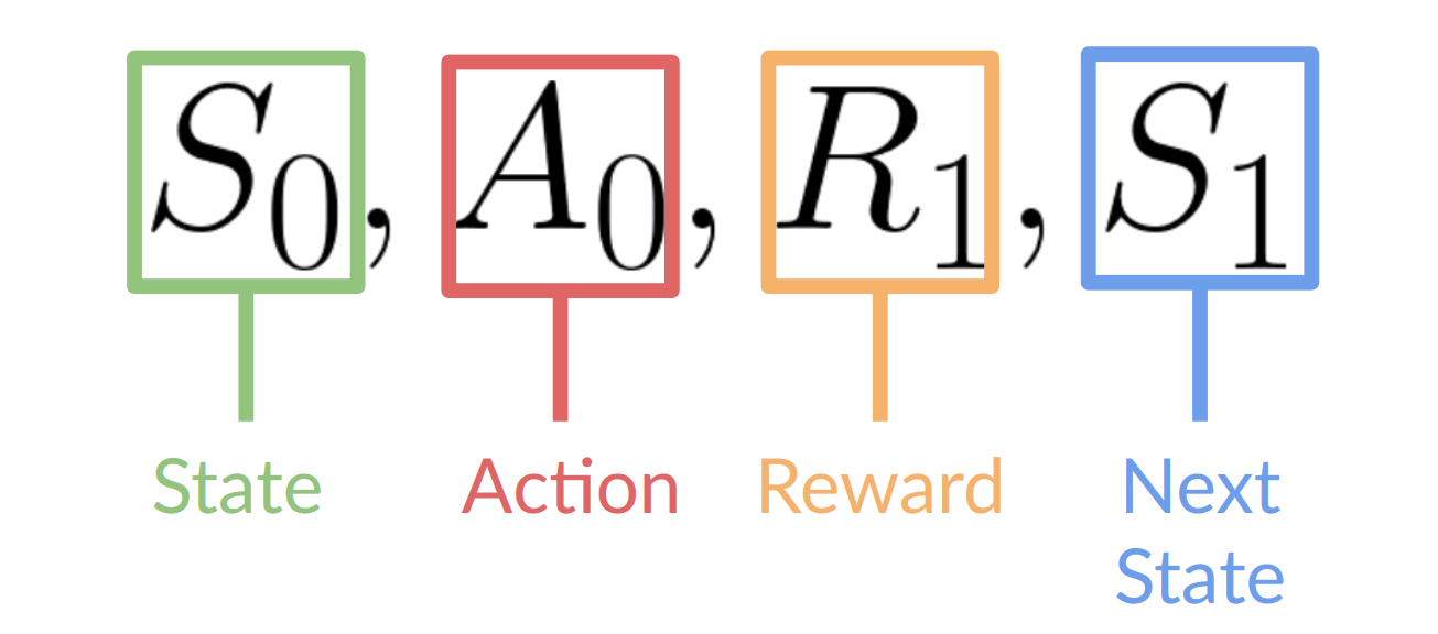
Figure to clarify the notations.

And as described above, the action taken by the agent on time \(t+1\) only depends on the reward and the state of time \(t+1\), which is the new state and reward gained through the action taken right before, i.e. \(A_t\). This is called the Markov Decision Process (MDP), simply put, the agent only needs the current state to decide the best action and neet not the history of all states seen before.

Naturally, the goal of reinforcement learning becomes maximizing the expected cumulative reward.

We can try to assert that the expected cumulative reward can be written as:

\[R(\tau)=\sum^{\infty}_{k=0}r_{t+k+1}\]

where \(\tau\) is the trajectory of the state and actions throughtout time like \(\tau=(s_0,a_0,s_1,a_1,...)\).

Keep in mind that since the reward into the future is less likely to occur, we introduce a discount factor to the individual reward, called gamma (\(\gamma\)) that is between \(0\) and \(1\).

So the adjusted expected cumulative rewards becomes:

\[R(\tau)=\sum^{\infty}_{k=0} \gamma^t r_{t+k+1}\]

Demystifying Policy in RL

We noted that the goal of RL is to build an RL agent that can select the actions that maximize its expected cumulative reward.

Then how can a model decide which action to take when given a state? -> policy \(\pi_\theta\).

We can define the “policy” as a parameterized function with respect to \(\theta\) and returns the most optimal action.

\[\text{state}\rightarrow\pi(\text{state})\rightarrow\text{action}\]

So naturally our goal becomes to optimizing the policy of the model through training, to get \(\pi^*\), that maximizes the expected reward.

There are mainly two ways to train the RL agent:

Policy-based optimization: teaching the agent which action to take given the state. It’s direct.
Value-based optimization: teaching the agent which state is more favorable so the agent takes actions that lead to more favorable states. Indirect.

Since the method that we are curious about today, GRPO, is a policy-based method, let’s talk a bit more about policy-based optimization.

Policy-Based Methods

Simply put, we are optimizing the policy for the agent which can map each environment state to the best corresponding action. This is deterministic, so we can also define a stochastic function that can map each state to a distribution of possible actions.

Deterministic: \(a=\mu_\theta(s)\). Same state will yield same action.
Stochastic: \(a\sim\pi_\theta(A\|s)\) is the proabability of taking action \(a\) over probability distribution of the set of possible actions \(A\), given the state.

Now, that we established the policy function, we can write the expected return \(J(\theta)\) as:

\[J(\theta)=E\big[\sum^T_{t=0}R(s_t,a_t);\pi_\theta\big]=\sum_\tau P(\tau;\theta)R(\tau)\]

where \(P(\tau;\theta)\) is the probability of \(T\)-step trajectory \(\tau\), given \(\theta\).

Since our goal is to maximize \(J(\theta)\), the optimal policy \(\pi^*\) can be expressed as:

\[\pi^*=arg\,max_\theta J(\theta)\]

Policy Gradient

Great, but how do we actually find this optimal policy \(\pi^*\)?

Assuming that you are familiar with gradient descent, we can apply almost exactly the same method for policy optmization!

We could update our policy by applying gradient to its parameter \(\theta\) as such:

\[\theta_{t+1}=\theta_t+\alpha\nabla_\theta J(\theta)\]

The term \(\nabla_\theta J(\theta)\) is the policy gradient.

To make \(J\) differentiable, let’s rewrite our objective function \(J\) as:

\[J(\theta)=E[r(\tau)]=\sum_\tau P(\tau;\theta)R(\tau)=\int\pi_\theta(\tau)r(\tau)d\tau\]

over a continuous trajectory \(\tau\).

Now, the policy gradient becomes:

\[\nabla_\theta J(\theta)=\int\nabla_\theta\pi_\theta(\tau)r(\tau)d\tau=\int\pi_\theta(\tau)\nabla_\theta\log\pi_\theta(\tau)r(\tau)d\tau=E[\nabla_\theta\log\pi_\theta(\tau)r(\tau)]\] \[\because \nabla_\theta f(x) = f(x)\nabla_\theta\log f(x) \text{ and } E[f(x)]=\int p(x)f(x)dx\]

We can take out \(r(\tau)\) as a constant since its value does not directly depend on the parameters, which makes sense.

Let’s differentiate \(\log\pi_\theta(\tau)\):

We know that

\[\pi_\theta(\tau)=\pi_\theta(s_1,a_1,...,s_T,a_T)=p(s_1)\Pi^T_{t=1}\pi_\theta(a_t,s_t)p(s_{t+1}|a_t,s_t)\]

Taking a \(\log\) on both sides,

\[\log\pi_\theta(\tau)=\log p(s_1)+\sum^T_{t=1}\big[\log\pi_\theta(a_t|s_t)+\log p(s_{t+1}|a_t,s_t)\big]\]

Taking the gradient on \(\theta\),

\[\nabla_\theta\log\pi_\theta(\tau)=\sum^T_{t=1}\nabla_\theta\log\pi_\theta(a_t|s_t)\]

Therefore, the final policy gradient equation using sampling yields:

\[\nabla_\theta J(\theta) = E[\nabla_\theta\log\pi_\theta(\tau)r(\tau)] \approx \dfrac{1}{N}\sum^N_{i=1}\Big[\big(\sum^T_{t+1}\nabla_\theta\log\pi_\theta(a_{i,t}|s_{i,t})\big)\big(\sum^T_{t=1}r(s_{i,t},a_{i,t})\big)\Big]\]

And use this gradinet to update our policy:

\[\theta_{t+1}=\theta_t+\alpha\nabla_\theta J(\theta)\]

PPO (Proximal Policy Optimization)

The idea with Proximal Policy Optimization (PPO) is that we want to improve the training stability of the policy by limiting the change you make to the policy at each training epoch: we want to avoid having too large of a policy update.

For two reasons:

We know empirically that smaller policy updates during training are more likely to converge to an optimal solution.
A too-big step in a policy update can result in falling “off the cliff” (getting a bad policy) and taking a long time or even having no possibility to recover.

PPO updates the policy conservatively. We can measure how much the policy has changed compared to the former one using a ratio and clip this ratio within range \([1-\epsilon, 1+\epsilon]\). This prevents the new policy from deviating too much from the old one (hence the proximal policy term).

We can rewrite our policy objective function as follows:

\[L^{\text{PG}}(\theta)=E_t[\log\pi_\theta(a_t|s_t)*A_t]\]

where \(A_t\) denotes the “advantage” this action has over other actions at that state and \(L^{\text{PG}}\) is the loss function that’s being optimized. Advantage is defined as: \(A_t=Q(s_t,a_t)−V(s_t)\)

where:

The term \(Q(s, a)\) is the action-value function, which estimates the expected return (cumulative future reward) when taking action ‘a’ in state ‘s’ and following the current policy thereafter.
The term \(V(s)\) is the state-value function, which estimates the expected return when starting in state ‘s’ and following the current policy.

Denote the ratio between the old and new policies as:

\[r(\theta)=\dfrac{\pi_\theta(a|s)}{\pi_{\theta_\text{old}}(a|s)}\]

From this, we can deduce that if \(r(\theta)>1\), the actions \(a_t\) at state \(s_t\) is more probable under the new policy \(\pi_\theta\), and magnitude of the ratio shows the divergence of the new policy from the old one.

With PPO’s clipping, the objective function becomes:

\[L^{\text{CLIP}}(\theta)=E_t[\min(r_t(\theta)A_t, \text{clip}(r_t(\theta),1-\epsilon,1+\epsilon)A_t)]\]

We can replace the log probability with the policy ratio to have similar effects of the original policy gradient loss function while staying more conservative with the aid of clipping.

GRPO (Group Relative Policy Optimization)

Abstract from the Deepseek Paper:

Mathematical reasoning poses a significant challenge for language models due to its complex and structured nature. In this paper, we introduce DeepSeekMath 7B, which continues pre-training DeepSeek-Coder-Base-v1.5 7B with 120B math-related tokens sourced from Common Crawl, together with natural language and code data. DeepSeekMath 7B has achieved an impressive score of 51.7% on the competition-level MATH benchmark without relying on external toolkits and voting techniques, approaching the performance level of Gemini-Ultra and GPT-4. Self-consistency over 64 samples from DeepSeekMath 7B achieves 60.9% on MATH. The mathematical reasoning capability of DeepSeekMath is attributed to two key factors: First, we harness the significant potential of publicly available web data through a meticulously engineered data selection pipeline. Second, we introduce Group Relative Policy Optimization (GRPO), a variant of Proximal Policy Optimization (PPO), that enhances mathematical reasoning abilities while concurrently optimizing the memory usage of PPO.

Group Relative Policy Optimization (GRPO) is a variant of PPO specifically designed to improve mathematical reasoning capabilities while being more memory-efficient than standard PPO. The key innovation lies in how it handles the advantage calculation and policy updates.

The Core Problem with Standard PPO for Reasoning

In standard PPO, we calculate advantages for individual state-action pairs. However, for complex reasoning tasks like mathematics, this approach has limitations:

Individual action evaluation: Each step in a reasoning chain is evaluated independently
Memory overhead: PPO requires storing value function estimates for every state
Sparse rewards: Mathematical problems often have sparse rewards (only at the end when the answer is correct/incorrect)

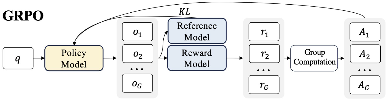
GRPO’s Key Innovation: Group-Based Advantage Instead of computing advantages for individual actions, GRPO groups related samples and computes relative advantages within each group. Here’s how group-based advantage works:

Grouping Strategy
- For each training step, the model will generate a set of \(G\) completions for each prompt denoted as \(o_i\), which are multiple solution attempts for the same problem
- Each group contains different reasoning paths or approaches to solve the same mathematical problem
- This allows the model to learn from comparing different solution strategies
For each of the \(G\) sequences, we compute the reward using a reward model.
Relative Advantage Calculation Rather than using the standard advantage formula, GRPO computes advantages relative to the group with \(A_t^\text{GRPO}=R_t−\bar R_\text{group}\) where:
- Reward \(R_t\) is the reward for the current trajectory
- Mean reward \(\bar R_{\text{group}}\) is the average reward within the group
Optimization
- The policy tries to maximize the GRPO objective, which includes the calculated advantages and a KL divergence term.

GRPO Objective

alt text

GRPO objectivce calculation (from HuggingFace).

We need to introduce the KL divergence term:

\[D_{\text{KL}}[\pi_\theta||\theta_\text{ref}]=\dfrac{\pi_{\text{ref}}(o_{i,t}|q,o_{i,<t})}{\pi_{\theta}(o_{i,t}|q,o_{i,<t})}-\log\dfrac{\pi_{\text{ref}}(o_{i,t}|q,o_{i,<t})}{\pi_{\theta}(o_{i,t}|q,o_{i,<t})}-1\]

The KL Divergence measures how one probability distribution differs from another, which can be used to preventing large policy changes. The reference policy \(\pi_\text{ref}\) is often the initial supervised finetuned model.

While we want the model to make compliant updates (close to the reference policy), we also want to maximize the advantage. The GRPO loss can be constructed as follows:

\[L_\text{GRPO}(\theta)=-\dfrac{1}{\sum^G_{i=1}|o_i|}\sum^G_{i=1}\sum^{|o_i|}_{t=1}[\dfrac{\pi_{\theta}(o_{i,t}|q,o_{i,<t})}{[\pi_{\theta}(o_{i,t}|q,o_{i,<t})]_{\text{no grad}}}\hat A_{i,t}-\beta D_{\text{KL}}[\pi_\theta||\pi_{\text{ref}}]]\]

Breaking it down:

\(L_{\text{GRPO}(\theta)}\) - The GRPO loss function we’re trying to minimize, parameterized by \(\theta\) (the model parameters)

Outer Summation Components

\(G\) - Number of groups (GRPO processes data in groups/batches)
\(\|o_i\|\) - Size of group i (number of sequences in that group)
\(\sum^G_{i=1}\) - Sum over all G groups
\(\dfrac{1}{\sum^G_{i=1} \|o_i\|}\) - Normalization factor (dividing by total number of sequences across all groups)

Inner Summation

\(\sum^{\|o_i\|}_{t=1}\) - Sum over all sequences in group \(i\) (from sequence 1 to \(\|o_i\|\))

Core Policy Terms

\(\pi_\theta(o_{i,t} \| q, o_{i,<t})\) - Current policy probability of generating token \(o_{i,t}\) given:
- \(q\) - The input query/prompt
- \(o_{i,<t}\) - All previous tokens in the sequence \((o_{i,1}, o_{i,2}, ..., o_{i,t-1})\)
- \(\theta\) - Current model parameters being optimized
\([\pi_\theta(o_{i,t} \| q, o_{i,<t})]_\text{no grad}\) - Same as above but with gradients stopped (detached from computational graph)

Advantage and KL Terms

\(A_{i,t}\) - Advantage estimate for token \(t\) in sequence \(i\) of group \(i\). This captures how much better/worse this token is compared to the expected value
\(\beta\) - Hyperparameter controlling the strength of the KL regularization
\(D_\text{KL}[\pi_\theta \| \pi_\text{ref}]\) - KL divergence between:
- \(\pi_\theta\) - Current policy being trained
- \(\pi_\text{ref}\) - Reference policy (typically the initial SFT model)

Sequence Indexing

\(o_{i,t}\) - The \(t\)-th token in sequence \(i\)
\(i\) - Group index (1 to \(G\))
\(t\) - Token position within sequence (1 to \(\|o_i\|\))

A visualization might help:

alt text

In short, the first term represents the scaled advantage and the second term penalizes deviations from the reference policy. The equation essentially computes a weighted average of policy gradients across all tokens in all groups, with the advantage term guiding the direction of updates and the KL term preventing the policy from deviating too far from the reference policy.

There are other variants of loss functions for GRPO, feel free to explore!

Final Remarks

A quick summary:

LLM training follows pretraining → finetuning → RLHF sequence where post-training uses reinforcement learning
Agent learns optimal behavior by taking actions in environment to maximize cumulative reward through trial and error
Policy (\(\pi_\theta\)): Parameterized function that maps environment states to optimal actions or action probability distributions
Objective: Find optimal policy \(\pi^*\) that maximizes expected return \(J(\theta)\) using policy gradient methods
Advantage \(A_t\): Measures how much better an action is compared to average expected value at that state
Main idea behind PPO: Clip policy ratio within \([1-\epsilon, 1+\epsilon]\) range to ensure conservative, stable policy updates
GRPO: Uses group-based advantage calculation by leveraging multi-completions for each prompt and computing relative advantages within the groups

GRPO optimizes for correct reasoning outcomes rather than just predicting next tokens, which improves mathematical problem-solving abilities. By allowing the model to compare different reasoning strategies and learn from relative quality of solutions boosts the model’s reasoning performance over the course of the RL process.

References

Thank you.